You can do this assignment in any language you like, with either Matlab or C/C++ together with the vision lab support code being the two recommended choices. Python might be up to the task also, but you will have to sort out numerical library support on your own (or as a group).

Those (considering) working with the vision lab should do at least some of the assignments in C/C++.

Information for those working in C/C++.

Assignment specification

This assignment has three parts. The second part is only required for grad students. Modest extra credit is available to undergraduates who do some of the grad student part.

To simplify things, you should hard code the file names in the version of your program that you hand in. You can assume that the grader will run the program in a directory that has the input files.

Specific deliverables are flagged with (+).

Part A

    /cs/www/classes/cs477/fall11/ua_cs_only/assignments/rgb_sensors.txt 

For this assignment you need to write a program which does the following.

1. Generate 1600 random light spectra as 101 element row vectors. The standard random number generator is fine. (The spectra need to be positive). To make grading and debugging easier, precede your call to rand() with a call to rng() with the argument 477 (i.e., rng(477)). Convince yourself that your experiments are repeatable. (C users can use kjb_seed_rand(477, 577));

   Note that rng() is not available on older versions of Matlab, including the ones on gr01-gr08 before Sept 12, 2011.

2. Compute the (R,G,B) responses for the 1600 light spectra.

   The standard random number generator provides values of the order of one, but if you make it into a light spectra vector, you are pretending that someone measured these values. But what are the units? You understand that there is an arbitrary scale factor implicit in your light spectra because of the arbitrary range of [0,1]. So, you can pretend that your light spectra are some constant, K, times real spectra in physical units. (In practice we often ignore this scale, as the absolute intensity of light is often somewhat arbitrary anyway (e.g., its units are a consequence of the photographer adjusting the aperture), but you should understand that it is there).

   Similarly, the provided sensitivity curve that has implied units. They come from a calibration experiment for a particular spectrophotometer, and it converts spectra, as measured by the by that instrument, into RGB for the camera settings used on the day of the experiment. To be specific, the numbers would have to be of the order of 1e-4, not the order of 1.0 as given by rand(), to have RGB values in the range (0,255).

   The bottom line is that you do not necessarily expect to get sensor responses in the range of (0,255) unless we had adjusted the sensors before hand to make that so. Determine a scale factor, K, that scales (multiplies) your 1600 (R,G,B) so that the maximum of any of the (R,G,B) is 255. (You do not need to report this value).

   Multiply the randomly generated light spectra by K, and regenerate the (R,G,B). Verify that the max R,G,or B is now 255.

   To visualize the (R,G,B) so the instructor can easily see the data, we will pretend that the 1600 spectra can from the squares on a 40 x 40 grid. The first 40 spectra correspond to the first row, the second 40 to the second row, and so on. We will create an image that we would expect if each of the squares occupied 10 x 10 pixels.

   Specifically, create a 400 by 400 color image made from 1600 10x10 blocks of uniform RGB. The RGB of the 40 blocks in the first row should be the first 40 RGB values you have generated, the next row should have the next 40 values, and so on.

   Your computer program should display this image (+).

   Hint: If your image is not what you expect, check the data types. You may have to cast the values to create an image for display..

3. Now simulate measurement error by adding a differnt amount of random noise to each of the (R,G,B) values for each of the 1600 colors. Start with noise of the order 10. Since you scaled the data to (0,255), this is about 2%.

   (More specifically, generate random numbers in [-10,10] and add them to your (R,G,B).

4. You now have a simulation of a camera calibration experiment. You have light spectra, and you have a bunch of responses with some noise. Use the least square method developed in class to estimate the camera sensitivities.
5. Plot the "real" sensors and the estimated ones on the same plot. (+).

Part B (only required for grad students).

    /cs/www/classes/cs477/spring08/ua_cs_only/assignments/light_spectra.txt

    /cs/www/classes/cs477/spring08/ua_cs_only/assignments/responses.txt 

1. Estimate the camera sensitivities using this data. Again plot the real sensors and the estimated ones on the same plot. (+).
2. Hopefully you will find that your sensors are terrible! Can you explain this (in the README (+))? Consider that the real light spectra came from a limited number of sources, through a limited number of filters, hitting a limited number of surfaces. Further, the reflectance spectra of most surfaces is smooth, which implies that they have limited dimension. For example, you can reconstruct them from a small set of sines and cosines (Fourier series).
3. We can make things better by doing constrained least squares. For example we can insist that the solution vector is positive. Implement this. If you are doing this in Matlab, you will need to use a function like quadprog. (The way quadprog() is set up is a little different than what you might expect. Here is a link to a simple example if you are having trouble. If you are using the UA vision library (KJB library), then you will want to look at the man page for constrained_least_squares Again, plot the results (+) together with the real sensors.
4. Hopefully you will now have positive sensors, but they are still weird. The problem is that they are not smooth. We can promote smoothness by pushing the derivative of the sensor curve towards zero. In this paradigm, this amounts to introducing equations that set the derivative to zero, and thus increasing deviations from perfectly smooth lead to greater error that is traded off with the error of fitting (which we are already using). Before reading on, consider how you might arrange this.

   OK, I am assuming that you have thought about this, and want to check your ideas. Consider a matrix that implements a derivative operator, which, when using vectors to represent functions, can be approximated using successive differences. If the matrix M does that to a vector R, then D given by D=M*R is a vector where

           D    =    R      - R 
            i         i+1      i
   

   If we M*R = 0, we can promote smoothness on R. You should ignore fence post problems (i.e. you can compute 100 differences for a 101 element spectra).

   Further, introduce a scalar multiple of the above differencing matrix which we will refer to as lambda. You will tweak lambda below.

   We want a smooth function, so we want the differences to be small. In least squares, this means that we want them to be (approximately) zero. Augment your light_spectra matrix with another 100 rows that is the differencing matrix. Augment your response (R,G,B) matrix to have the desired result (zero).

   Verify for yourself that tweaking lambda adjusts the balance of fit and smoothness. You should be able to produce very smooth curves that do not resemble your sensors, and curves approaching the ones you found in the previous part, where lambda == 0 should give exactly the same sensors as before. Provide plots for 5 different ascending values of lambda to illustrate the control you have on the output. Make sure that you have two for lambdas that you consider too small, and two for lambdas that you consider too large. The third plot should be a value of lambda that you think is pretty good. Note that the curve for blue (leftmost, covering the smaller wavelengths) cannot be fit very well. Don't worry about this.

   Provide five plots (+). All plots should have both the real sensors and the estimated ones on them. The plots should have the value of lambda in the title.

   Note: Lambda implements the desired effect because in least squares any row can be weighted by simply multiplying both the row and the response by a scalar. Think about the error function and make sure you understand why this works.

Part C

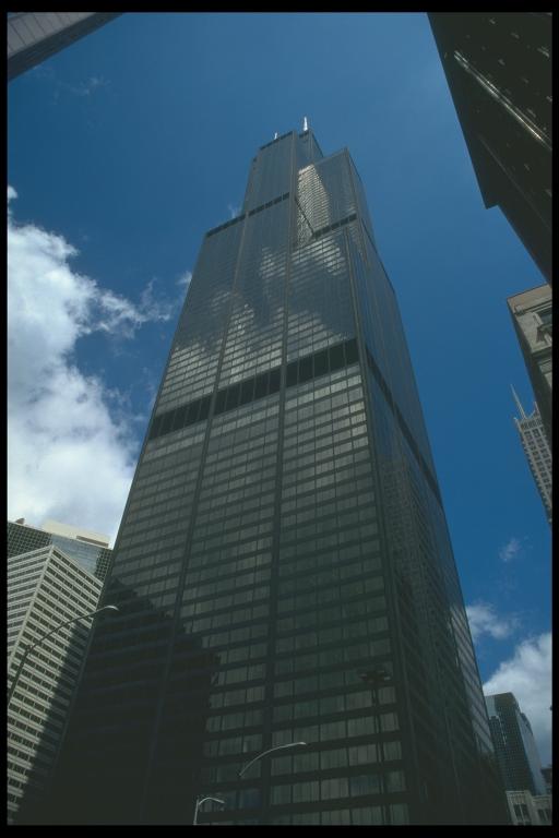
Below are links to two images. Dump these into a into a drawing program, and draw enough lines over the image to make a case that the image is either approximately in perspective or not. (Have a look at the building examples in the lecture notes if this is not making sense). You should understand and state your assumptions, and explain your reasoning. To get you started: You can assume that that the chandelier is perfectly symmetric.

Your deliverables for this part of the assignment should be a PDF with your images with lines drawn on them and an explanation of what you conclude.

For the chandelier image, you must also put small circles (i.e., "dots") that make it clear where the lines come from. In the case of the building, it will be generally clear how you drew the line, bu in the case of the chandelier image this will not be the case. Help the grader by showing the points that you are drawing lines through. If you color code the points and/or lines, this will help provide points of reference in your explanation.

Image one

Image two

Part D (Optional challenge problems)

In class we learned that under perspective projection, parallel lines (generally) converge to a point. Can you prove this?

We also learned that under perspective projection, the vanishing points for sets of coplaner parallel lines are colinear. Can you prove this?

What to hand in

If you are working in Matlab: You should provide a Matlab program named hw2.m, as well any additional dot m files if you choose to break up the problem into multiple files.

If you are working in C/C++ or any other compiled language: You should provide a Makefile that builds a program named hw2, as well as the code. The grader will type:

    make
    ./hw2

If you are working in any other interpreted/scripting language: Hand in a script named hw2 and any supporting files. The grader will type:

    ./hw2

You should also hand in a README explaining which of the 3 options apply (i.e., how to run your program), and answers to any questions posed about the code. In particular, for this assignment, grad students should try to answer the question regarding the cause of the messy pseudoinverse fit.

Finally, you need to hand in a PDF question C.

To hand in the above, use the turnin program available on lectura (turnin key is cs477_hw2).

For those not familiar with turnin:

To hand in files using turnin you need to sign onto machine lectura, and make sure that the files you want to hand in are in a directory that lectura sees, and then change to that directory. Note that your home directory on the graphics machines and lectura is the same, so if you have just tested your program on a graphics machine, you have probably done all the file transferring that you need to do. To hand in file XXX, you would do the following:

turning cs477_hw2 XXX

For more detailed instructions, use:

    man turnin