Due: Friday, February 19, 2010 (TA will not look at them before Saturday morning).
Credit: Approximately 8 points (Relative, and very rough absolute weighting)
It is probably a bit easier in Matlab, but doing some of the assignments in C may prove to be a useful exercise. If you think that vision research or programming may be in your future, you might want to consider doing some of the assignments in C/C++. If you are stretched for time, and like Matlab, you may want to stick to Matlab. Your choice!
Information for those working in C/C++. (Updated for this assignment).
This assignment has four parts, three of which are required for undergrads.
To simplify things, you should hard code the file names in the version of your program that you give to the TA.
The file
/cs/www/classes/cs477/spring06/ua_cs_only/assignments/line_data.txt
is an ASCII file containing coordinates of points that are assumed to lie on a
line. Apply the two kinds of least squares line fitting to the data. You need to
implement the fitting yourself based on formulas given in class.
[ There may be Matlab routines that simplify this question (e.g. REGRESS), but you need to use slightly lower level routines to show that you understand how things are computed. However, you may find it interesting to compare with the output of REGRESS or like routines. ]
Your program should fit lines using both methods, and create two plots showing the points and the fitted lines. For each method you should output the slope, the intercept, and the error of the fit under both models (eight numbers total). Comment on how do you expect that the error under the one model to compare with the error of the line found by the alternative model, and vice versa.
Overview. In part B, you will calibrate a camera from an image of a coordinate system. You will use that image to extract the image location of points with known 3D coordinates by clicking on them. The camera calibration method developed in class will then be used to estimate a matrix M that maps points in space to image points in homogeneous coordinates. Having done so, you will be able to take any 3D point expressed in that coordinate system and compute where it would end up in the image. This applies, of course, to the points that you provided for calibration, and the next step is to visualize and compute how well the "prediction" of where the points should appear compares to where they should appear.
(Note that the following parts of this assignment will not work out accurately. You are purposely being asked to work with real, imprecise data that was collected quickly).
Use the first of these images
|
IMG_0862.jpeg
(tiff version)
|
(tiff versions are supplied in case there are problems with the jpeg versions or the compression artifacts are giving you trouble, but note that the tiff versions are BIG!) |
To get the pixel values of the points, you need to either write a Matlab script to get the coordinates of clicked points, or you can use the program kjb_display (PATH on graphics machines is ~kobus/bin/linux_x86_64_c2, MANPATH ~kobus/doc/man) which is a hacked version of the standard, ImageMagick version of "display", or you can use some other software that you may know of. If you use kjb_display, use alt-D to select data mode. Then the coordinates of pixels clicked with the third button are written to standard output.
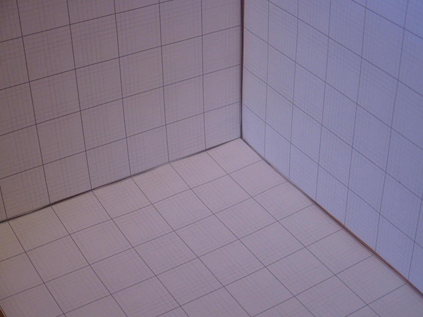
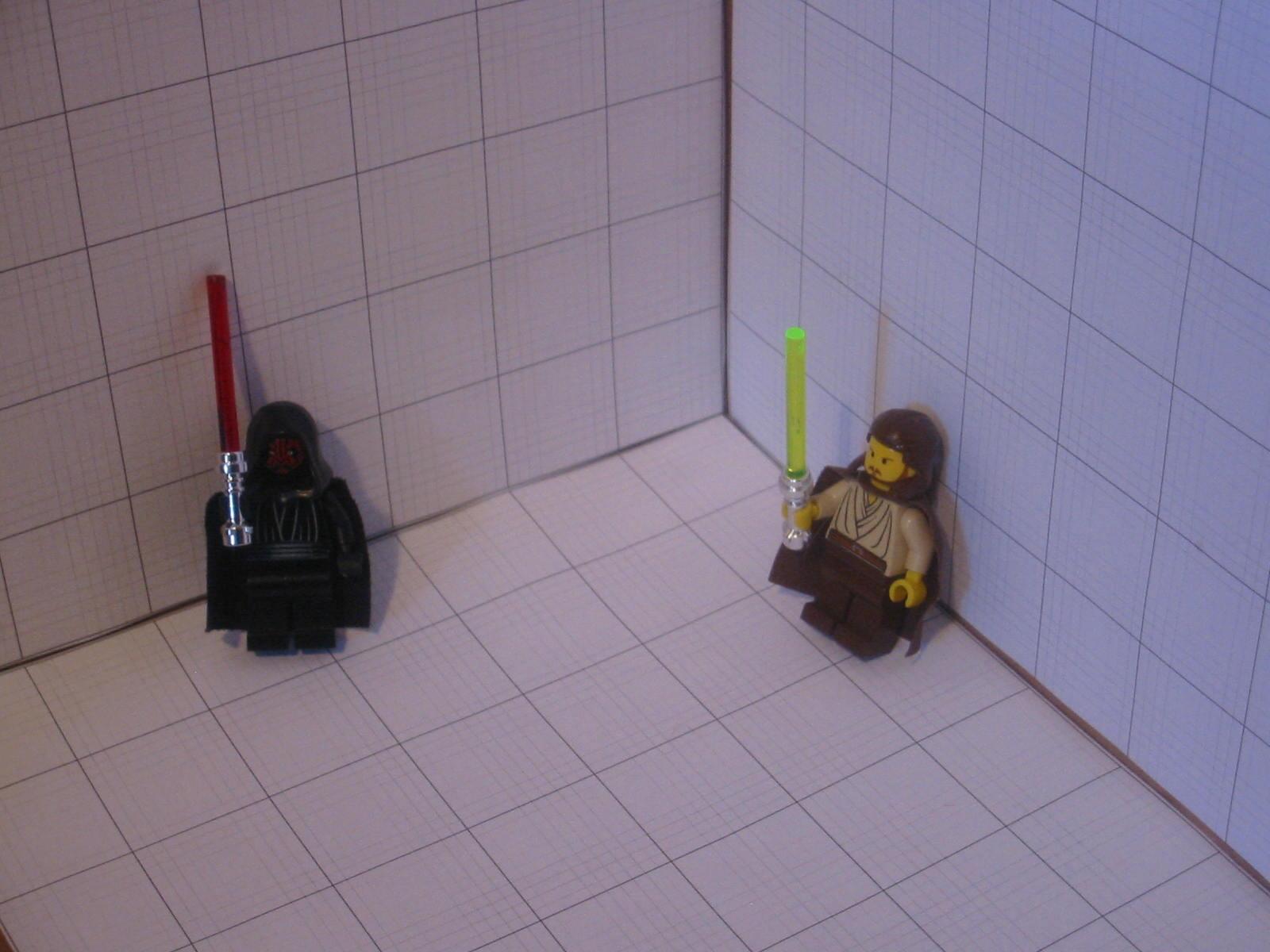
To set up a world coordinate system, note that the grid lines are 1 inch apart. Also, to be consistent with the light direction given later, the X-axis should be the axis going from the center leftwards, the Y-axis is going from the center rightwards, and the Z-axis is going up. (It is a right handed coordinate system).
Using the points, determine the camera matrix (denoted by M in class) using linear least squares. Report the matrix.
Using M, project the points into the image. This should provide a check on your answer. Provide the TA with an image showing the projected points.
Finally, compute the squared error between the projected points and where they should have gone (i.e., where you found them by clicking). This is an error estimate corresponding to the projection visualization just discussed.
Question: Is this the same error that the calibration process minimized? Why? Comment on whether is this good or bad.
Recall that in class we decided that M is not an arbitrary matrix, but the product of 3 matrices, one that is known, and the other two that have 11 parameters between them. Since there are 11 values available from M, this suggests that we can solve for those parameters. Let's give this a go!
Let's assume that the camera has perpendicular axes, so that we can assume that the skew angle is 90 degrees if needed. Use the equations on page 46 of the text to compute the extrinsic and intrinsic parameters of the camera. If you do not have the text, see the supplementary slides "intrinsic.pdf" .
In particular, you will recover the orientation and location of the camera, which will be used in the next part. Report your estimates.
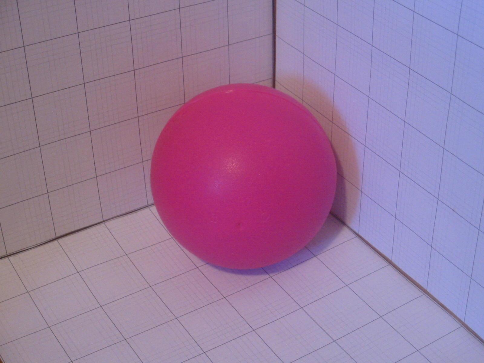
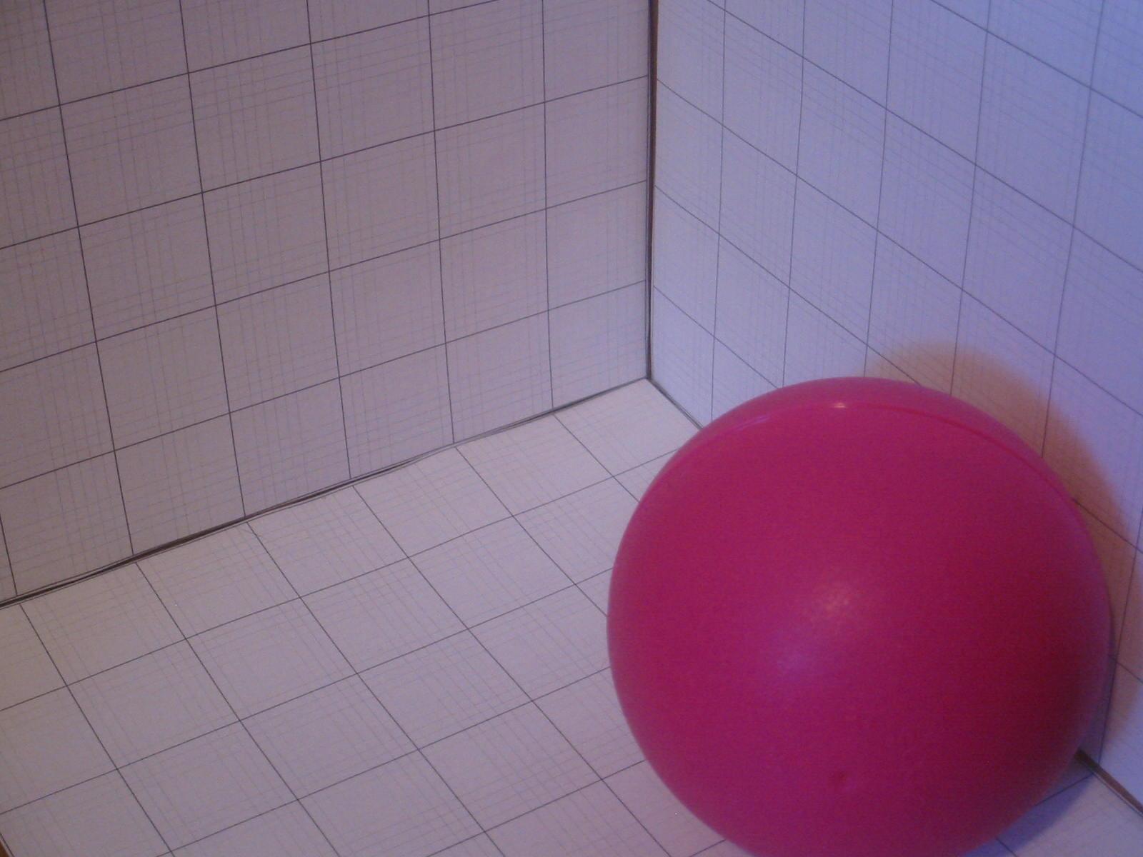
As a further direct check on the results, in this image (jpeg) (tiff version) the camera was 11.5 inches from the wall. This can be used to compute alpha and beta more directly.
Introduction: One of the consumers of vision technology is graphics. Applications include acquiring models for objects based on images, and blending virtual worlds with image data. This requires understanding the image. For example, if you create a graphics image, the camera location and parameters are supplied by some combination of hard coded constants, and user input. For example, the user may manipulate the camera location using arrow key. In the following part, we have a different situation. We want to use the camera that took the image. But we know how to do this (consult M).
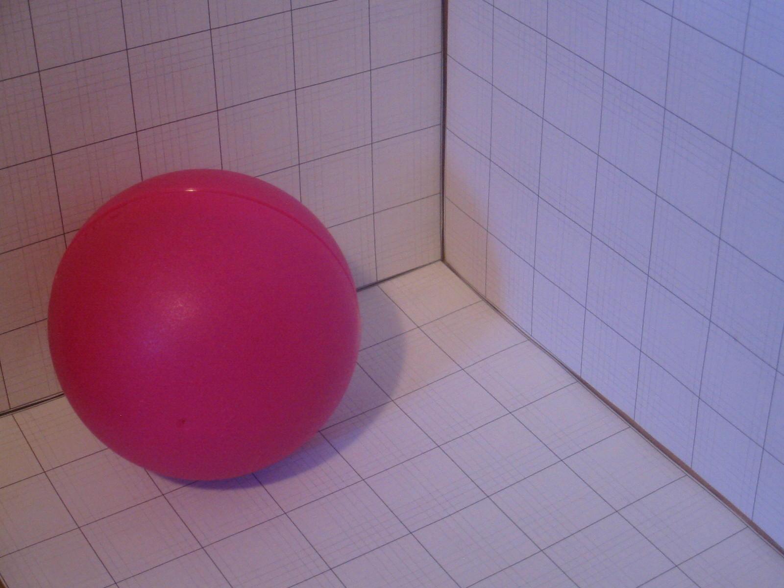
Now the task: Reportedly, the light was (roughly) at coordinates 33, 29, and 44. Ask yourself if this makes sense given the shading of the objects in the images that have objects. We now want to render a sphere into one of the images with one or more objects in it with plausible shading. Using the Lambertian reflectance model, render a sphere in the second image using any color you like. In order that this assignment does not rely on having taken graphics, we will accept any dumb algorithm for rendering a sphere (and we will provide help to those who want it). For example, you could model a sphere as:
x = x0 + cos(phi)*cos(theta)*R
y = y0 + cos(phi)*sin(theta)*R
z = z0 + sin(phi)*R
Now step phi from -pi/2 to pi/2 and step theta from 0 to 2*pi to get a bunch of 3D points that you will draw a sphere if projected into the image using the matrix, M. (If your sphere has holes, use a smaller step size).
There is one tricky point. We need to refrain from drawing the points that are not visible (because they are on the backside of the sphere). Determining whether a point is visible requires that we know where the camera is. The grad students will compute the location of the camera. The TA will mail a camera location to the U-grads (but you can guess a reasonable value).
Assume that the camera is at a point P. For each point on the sphere, X=(x,y,z), the outward normal direction for the point on the sphere can be determined (you should figure out what it is). Call this N(X). To decide if a point is visible, consider the tangent plane to the sphere at the point, and compute whether the camera is on the side of the plane that is outside the sphere. Specifically, if
(P-X).N(X) > 0then the vector from the point to the camera is less than 90 degrees to the surface normal, and the point is visible.
A) Add a specularity on the sphere.
B) Render the shadow of the sphere.
Note that these problems are not completely trivial For (A), you should develop equations for where you expect the specularity to be. You will need to consider the light position, the sphere, and the camera location. You may find it easiest to write the point on a sphere, X = X0 + R*n, where n is the normal which varies over the sphere.
To hand in the above, use the turnin program available on lectura (turnin key is cs477_hw3).