ISTA 352 - Images: Past, Present, and Future - Fall 2012

Assignment One

Due: Late (*) Friday, Sept 07.

(*) "Late" means that the instructor might start grading by 8AM Saturday. Once the instructor starts grading, no more assignments will be accepted.

10 points

This assignment should be done individually

 

One purpose of this assignment is to become familiar with some basic matrix and image manipulation and Matlab. Matlab is useful for exploring ideas and prototyping programs. It is a popular programming environment for computer vision and machine learning, especially for those who do not have lots of experience in C/C++ because it allows one to focus more on the problem and less on the code. It has significant drawbacks for writing large programs or when performance matters. It is also a "product" which needs to be purchased and installed before it can be used. Nonetheless, it is a useful tool which image students should be exposed to. Some future assignments may either require Matlab, or be optionally done in Matlab.

Matlab is available for personal use to UA faculty, staff and students. It can be downloaded from http://sitelicense.arizona.edu/matlab/ by any University of Arizona faculty, staff or student with a netid. The site-license includes MATLAB, Simulink, plus 48 toolboxes.

Matlab is also installed on the UA SISTA/CS linux machines (the path is /usr/local/bin). Normally, to begin, you just type "matlab" at the shell prompt. For example, you may want to use the machines in GS 930, either on-site, or remotely. If your DISPLAY environment is properly set, the default behavior is to start the GUI interface. Otherwise, you will get the command line interface. This GUI is required for some of this assignment. You may find that the GUI is slow to start up, and painfully slow to use over a slow connection. For a faster startup (but without some of the features needed for some parts of this assignment), you can try

         matlab -nodisplay -nojvm 

 

Deliverables

There is much in this assignment that does not need to be handed in, or the answer is a short program and not very interesting to read (but I still want to see it). To reduce confusion, the deliverables within questions are flagged with ($), and questions with no deliverables are flagged with (@).

 

This assignment has 15 questions, of which two are optional challenge problems which can be exchanged and/or done for modest bonus points, and three which have no deliverables. Hence ten questions required for full marks.

 

Remember, programming is time consuming, so start early!

 

 

1. @ Become familiar with Matlab (no deliverables).

Read this short Matlab tutorial and be aware of this longer Matlab primer . Alternatively, you could work through "Getting started" in the Matlab help GUI system. The complete documentation for Matlab is also available on the web as well as being scattered about in the various forms of help.

All Matlab commands are well documented with Matlab's help system which are available through the GUI, as well as through the command line interface. For example, if you want to know how the svd function works, type help svd. You can also get help on all the built in operators and even the language itself. Typing help gives a list of help topics.

Tip: You may want to turn on paging (more on) for reading help pages.

2. @ Basic vector and matrix operations (no deliverables).

Let

 

 

 

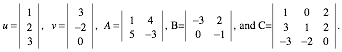
Work out the following by hand, and use Matlab to check your answers.

a)      u+v

b)     u-v

c)      u.v     (dot product)

d)      A+B

e)      A-B

f)      A*B

g)     C*u

3. Files and Paths

The interactivity of Matlab is great for debugging and experimenting, but usually one wants to type code into a file. But where is your file going to live? Assuming that you already know which directory (folder) that will contain your program, then you will find it easiest to run Matlab with that directory as the “working” directory. If you started up Matlab by typing “matlab” from that directory, then this is already the case. If you started up the Matlab GUI (e.g., by clicking an icon on the mac toolbar),  you will need to navigate to your directory, either using the GUI (“Current Folder” at the top), or using the command line. 

Tip: Matlab has pwd, ls, and cd commands that do what you expect.

Create a file hw1.m and put the following command in it to create the “hello world” program.

    fprintf('Hello world.\n');  

Tip: You can use any text editor you like to work on hw1.m,  including the one built into the Matlab GUI. To try that out, you can type:

    edit hw1.m

Check that it works by typing in hw1 at the Matlab prompt to execute the commands in the file. A file of this sort is known as a script. As you work through the exercises, update hw1.m with code that creates the required output. Your program should output headings demarking the questions ($), as well as helpful text explaining what is going on ($). If you want to break your program into modules, then include extra dot m files, but they should be called from hw1.m. Note that the deliverables flagged in this paragraph are part of the “exposition” part of the grade.”

4. Testing guesses

 

If two expressions are equal in general, then they have to be true for all randomly generated cases. While this is not “proof”, we can check our guesses to some extent in this way. If A and B are two equal matrices,  then norm(A-B)should be zero. Due to machine precision issues, it is possible that for our randomly generated cases, the computation results in a small number instead. For matrices with elements of the order of unity, we do not expect calculations to be more accurate than about one part in 10^15. (If this sort of issue interests you, you can find out more on Matlab’s interpretation of precision be entering “help EPS, or for more general information Google “IEEE floating point format”).

Write a program that uses random matrices of size 1 though 10, with both positive and negative elements in them, to verify, that at least in these cases:

(A*B)*C = A*(B*C)        (Formally, we say that matrix multiplication is associative).

 ($) Put your code into hw1.m so I can run it. Don’t forget to output helpful text such as a question separator and heading.

5. Reading and Displaying Images

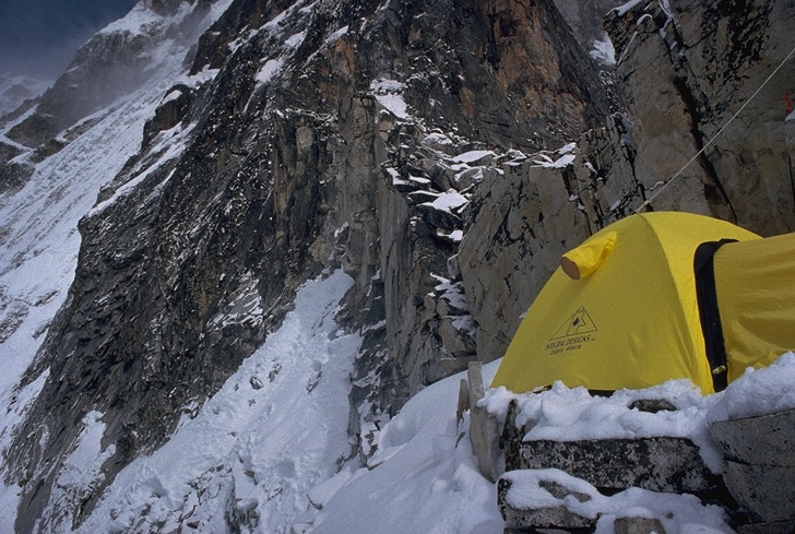
Place a JPEG color image in your working directory with the name 1.jpg. When I run your program, I will use this image:

 1.jpg  

If you want to use a different image, you should consider testing with that image as well before handing in your assignment.

Load the image (1.jpg) into a variable using imread. Type help imread to find out how to do this. Create a new figure using figure and display the image in it using imshow ($).

Tip: Make sure you put a semicolon at the end of your imread command! The semicolon at the end of a line prevents Matlab from displaying the result of an expression. Most of the time, you want the semicolon.

Make sure you understand the data structure being used to represent the image. Type whos to get a list of active variables along with their types and sizes. You can see that your image is a 3D array of bytes. This is row by column by "channel" where the channels are red, green, and blue intensity values.

What is the range of values contained in the image array? Use the min and max functions to output this information ($).

Hint: These commands by default operate on only one dimension of their argument. Convert your image into a 1D array (a vector) using the (:) notation when you pass it to min and max.

Hint for the hint: help colon.

Convert the image to grayscale using rgb2gray. Check the representation of the image now. Use size or whos to find this out. You will see that we now have a 2D array, which for Matlab, is a matrix. Create a new figure and display the black and white image ($).

6. Image channels

Create three grayscale images based on our color image by extracting the red, green, and blue pixels, respectively, into an array. Display the three images ($,$,$). Are they what you expect? Can you explain why some areas that are bright in the color image are dark in some of the grayscale "slices"?

Tip: While Matlab has C style loops, you should avoid doing this sort of thing with low level loops. Instead, use the colon notion (help colon).

Create a new color image that has the green channel from the original image as its red channel, the blue channel from the original as its green, and the red channel from the original as its blue. Create a new figure and display the result ($).

Hint: Again, you might find the colon notation helpful (help colon).

7. Visualizing Matrices

Convert the grayscale image into a double-precision type, and scale the values so that they lie in the range [0,1].

Hint: Use the double function to do the type conversion, and then divide by the maximum allowable value for a byte, which is 255.

Create a new figure using figure, and use imagesc to display the grayscale image in it. Why does it look so strange?! Type colorbar to find out. You can see that 0 maps to blue, 0.5 to green, and 1 to red. This is the default jet colormap that is useful for data visualization. For this example, we might prefer the grayscale colormap. Type colormap(gray) to do this.

Tip: Type help gray to see what default colormaps are available. Note that you can also make your own colormaps.

Tip: The imagesc command takes a second argument that lets you specify the range of values. By default, imagesc scales the data to use the full colormap, but this is not always what you want. In this example, we could add the argument [0 1] to the imagesc command would be a nop because that is the range we already scaled it it.

The image is probably distorted, i.e. the pixels aren't square. Use the axis command to fix this, and display a new figure ($).

Tip: When you display matrices as images, you usually want the axes to be scaled so that the pixels are square and the image not distorted. See help axis to determine how to do this. The axis image command is a useful one. You can also turn the display of the axes on and off with the axis command.

8. Histograms

 

A histogram divides up your data space into boxes, and puts counts of occurrences into them. They are visualizations of the empirical probability distribution of your data. (EG, how likely do very red pixels occur?). If you are not familiar with histograms, you should read the Wikipedia article and/or some other resource about them as we will assume that you know what they are.

Convert each of the three color channel "slice" images into 1D vectors and provide histograms for them with 20 bins for each of them ($,$,$) using the hist command.

9. Manipulating Matrices

In this section, we will work with the converted gray scale image with double values in the range [0,1].

Tip: Array indices in Matlab start at 1, not at 0 like C.

Tip: As in standard mathematical notation, the first index of a matrix is the row, and the second index the column. When viewing a matrix as an image, this means that the first index is the y direction going down, and the second the x direction going to the right. As is common with image manipulation tools, the origin is at the top left corner, the positive x axis points right, and the positive y axis points down.

Get the width and height of the image using size. The size function, as is common in Matlab, can return multiple arguments.

Hint: To store both the width and height into variables in one go, try [h,w]=size(im). You could alternately do h=size(im,1) and w=size(im,2).

Write a couple of nested for loops to set every 5th pixel, horizontally and vertically, to 1. This should set 1/25th of the pixels to white in a square lattice pattern. Create another figure and display this result in it ($).

Hint: Use the colon operator to define the limits of the for loops. See help colon and help for to see how to do this. Specifically, you want the minval:interval:maxval form.

Set all the same pixels to 0, making the ones that you just set to white become black. Do it this time without using any for loops. Create yet another figure and display this result in it ($).

Hint: You can index arrays in Matlab with vectors as well as with scalars, so im(Y,X)=0 will set multiple entries of im to zero when either X or Y are vectors, such as the vectors returned by the colon operator.

Hint on hint: What is described in the hint might take some getting used to. Like many things in Matlab, it is easiest to combine reading of the documentation with experimentation. It is helpful to try simple things on random matrices. To get a random square matrix of size 10x10 use rand(10), and to get one of size 4x12 use rand(4,12). Vectors can be created as follows:
v=[2 4 6 8];>
Given such tools in an interactive environment makes it easy to create vectors with integer values and see what happens when you use them as matrix indices in assignment statements.

Set all the pixels whose values are greater than 0.7 to zero. The command to do this is im(find(im>0.7))=0. Check that this works, create a new figure and display the result ) ($). You should understand why this works.

Hint: The (im>0.7) expression evaluates to a boolean matrix, which is true where the condition holds. The find function returns a vector containing the indices of the true values. This vector is then used to index the image and set all the values to zero. Why does this last step work when the matrix is 2D and the indexing is 1D? Matlab lets you treat matrices as 1D vectors too, linearizing the matrix in column-major order.

More on column-major order. Think for a moment how 2D arrays are stored in memory. There are a number of options. One options is that the array is stored as a linear sequence of numbers, i.e., a 1D vector. This still leaves two alternatives. One is that the first row is followed by the second row (row-major), which is how C/C++ handle fixed arrays. The second is that the first column is stored in order, followed by the second column, and so on. This is column-major order which is used by Fortran and inherited by Matlab. This is an important issue to understand for those that might want to call Fortran routines from C which is a useful skill!

@ More tricks (no deliverables)

Matlab makes it easy to write "vectorized" expressions without having to write for loops or if statements. For example, this will add all the values of the image:

sum(im(:))

The following will count the number of values greater than 0.9:

numel(find(im>0.9))

So will this:

sum(sum(im>0.9))

This will halve only those values greater than 0.9 (note the use of the .* operator to do element-size multiplication of matrices):

im = im - 0.5*im.*(im>0.9);

And so will this:

mask = (im>0.9);
im = im.*~mask + im.*mask*0.5;

This will set 100 unique random pixels to zero:

p = randperm(numel(im));
im(p(1:100)) = 0;

See help elmat for a list of interesting matrix manipulation and creation routines.

10. @ Writing Images (no deliverables)

Write the image to a file called out.jpg using the imwrite function. Use some independent image viewer like display, xv or a web browser to verify that this worked. If you are working on linux (not required in this course), I recommend learning about the ImageMagick suite of tools for converting, and displaying images (do "man convert", and a "man display" to find out more). Also the program import can be used to get a screen-shot in linux.

11. Camera sensors, light spectra, and plotting in Matlab.

 

The file linked here (rgb_sensors.txt), contains the three response function of the camera the instructor used for his dissertation work. The file linked here (light_spectra.txt),  has a variety of  light energy spectra as a function of wavelength. Both datasets contain vectors of 101 numbers which is a consequence of the instrument used to measure spectra which did so from 380nm to 780nm in increments of 4nm.

Study how to plot data,  and then make your program create a single plot showing the three sensitivity curves ($). Make sure that the first sensor’s line gets colored red, the second green, and the third blue. Next, plot the light spectra on a single plot ($). Describe the variety (or lack thereof) in a few sentences in your PDF writeup. Finally,  compute the RGB values predicted for the first 400 spectra and create an image of 20 by 20 blocks, each block being 20x20 ($). Each patch is what a white piece of paper would look like if it were illuminated by that light and captured by this camera.

12. In the previous question measurements were sampled at a high resolution of 101 points. Consider instead a single sensor described by seven wavelength regions, with relative sensitivities (1, 2, 3, 4, 3, 2, 1). (“7” is playing the same role as 101” was before). Provide a light spectra vector, based on the same seven wavelength regions which yields the value of  16 ($). Now provide a second light spectra vector which is different from the first which also yields 16 ($). Now provide a third light spectra different from the other two which also yields 16 ($). Comment on what the knowledge of the recorded sensor response (e.g., R or G or B in and image) tells you about the light spectra (assume you know the sensor sensitivity vector).

(This is not a programming assignment, although you are welcome to use Matlab to help with arithmetic. Do not hand in any code for it.

13. (*) (Remember “*” means challenge questions which are optional and/or substitutable). Consider the previous question, but now use the RGB sensors form the question before that. Find three different spectra which give the same RGB=(100, 150, 200) ($). How many linearly independent spectra do you think you could find that have the same RGB ($)? (If you like, you can ignore the constraint that light spectra need to be positive which complicates certain clean arguments you might make. On the other hand, if you can say something concrete about positivity, go for it!)

 

14. (*) After the epic on the second class with trying to project real time generation of movies in Matlab, I decided that in the future I would simply make movie files. I tested this by making movie files for our three demos which are now on the lecture web page. Interestingly, for movies of the order of 1,000 frames, I got ones that were of the order of 30-70MB. This seemed a bit big, but gzip reduced that by less then half. Getting to point: Focus on the unshuffling demo (demo one) and the defective modem demo (demo three), and consider that the original jpeg image was about 100KB. Thinking about how the movies were made, propose a close to lower bound estimate for the information content, defined by the number of bits needed to transmit the movie data to remote party ($). Having done that, lookup Kolmogorov complexity (the Wikipedia article is OK) and comment on whether your answer has anything to with that.

 

15. Documenting Functions in  Matlab

When you create a new function, it should always be documented so that help returns something informative. The convention in Matlab is to place the help message in comments after the function declaration (the comment character is "%").

For example, you can look at some of the code in the Matlab library. Some of it is implemented as .m files, and some of it is "builtin". Regardless, there should be a .m file for at least the documentation. Using the "which" command, see if you can find the .m file for your favorite function so far. On my mac, the path provided was not exact, but gave me a good idea where to look.

If you look at some of these examples, you will see that the first line of the comment contains a one-line description of the command. All subsequent contiguous comment lines are included in the help message. Document your hw1.mfunction in this style. For the purposes of this assignment, no need to be overly detailed. A short paragraph or two about the main teaching points will suffice ($).

 

What to Hand In

Hand in a Matlab program hw1.m and PDF write-up using the instructions linked here as a guide. Note that some of the exercises were just things that you should try---there is no corresponding code to hand in. Your PDF file should begin with meta-information such as which parts you substituted or did as extra questions, which questions you did not do or had a lot of trouble with, which language you used (Matlab), and which machine you tested it on (e.g., Mac laptop).

Specification summary: The instructor will change directory to where your assignment is, and then enter "help hw1" to see if you learned how to document Matlab files. They will then invoke your program with the command hw1, and check if the figures and results requested appear. You can scan for "$" to double check that you have it all.